Rubber Bands Tie Our Brains Together Too

Rubber bands in brains? Brief intro to graph representations and the mysteries behind spectral clustering.

People use hair bands to bundle up their messy hair all the time. As it turns out, this simple act of using elasticity is similar to a clustering approach that groups together messy data. Here, I’d like to show some cool brains as an introduction to spectral clustering, and explain how a popular clustering algorithm can be simply viewed as perturbations of rubber bands.

My lab is often curious about how the brain’s structure lead to function. In the case of human brains, the architecture of axons and their myelinated sheath facilitate the diffusion of water molecules along their main directions. By estimating the diffusion gradient in various ${x,y,z}$ directions, we can map out the underlying fiber structure that connects specialized brain regions of interest. The raw data is simply a bunch of estimated vectors in the ${x,y,z}$ directions:

\begin{Bmatrix}x_1 & x_2 & \ldots & x_n \\ y_1 & y_2 & \ldots & y_n \\ z_1 & z_2 & \ldots & z_n\end{Bmatrix}

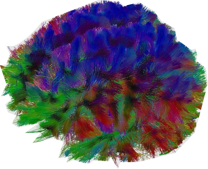
We can get artsy with these vectors and draw out all the fiber connections inside the brain by following the diffusion parameters voxel by voxel, publishers love these colorful images:

Instead of the colorful image, researchers work with a matrix of weighted scalars representing connection strength between pairs of brain regions:

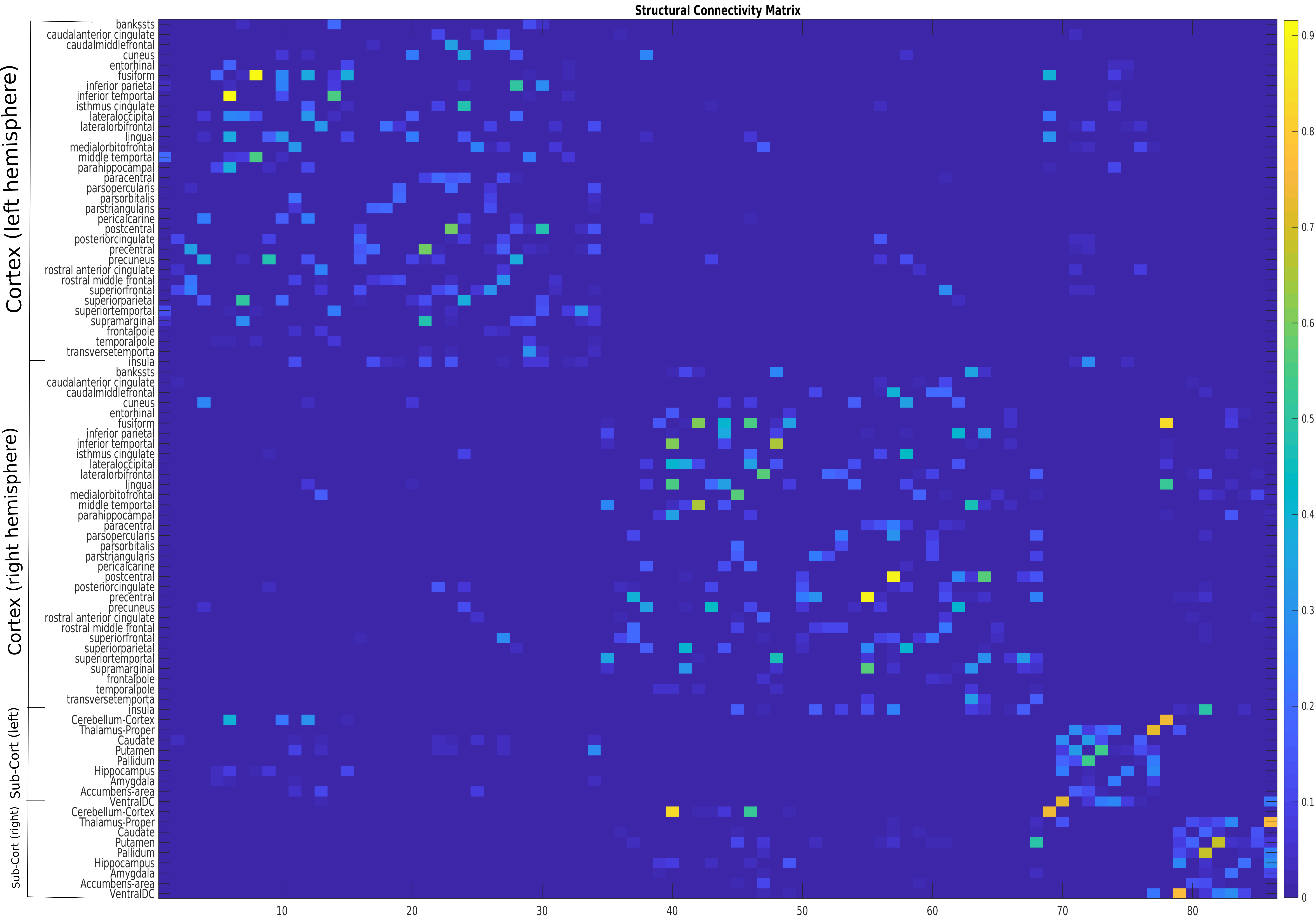
The obvious flaw in this matrix is that there is no spatial information about the data points. We only know the connection strengths between regions, but we do not know the location of each brain region, and we have no coordinate system defining the relative distance between each adjacent brain region. While this is a fatal weakness in our data, by utilizing rubber bands, i.e., spectral clustering, we can group these data points onto a brain without spatial information.

Basic graph representation and graph notation

Given this set of $N$ brain regions $x_1, …, x_N$ and connection strength $c_{i,j} \geq 0$ between all pairs of brain regions $x_i$ and $x_j$, we can transform this data into a simple representation on a graph: $G = (V,E)$. Each node $V_i$ in this graph ($G$) represents a brain region $x_i$. Two nodes are connected if the connection strength $c_{i,j}$ between the brain regions $x_i$ and $x_j$ is bigger than zero (or a threshold), then the edge (E) between the two nodes is weighted by $c_{i,j}$.

Additionally, for each node/vertex $V_i \in V$ (English: $V_i$ inside of V), we define the degree of that node as the sum of the weights to adjacent nodes: $d_i = \sum_{j=1}^{N} c_{i,j}$.

And the degree matrix $D$ is defined as an N-dimensional diagonal matrix where the degrees $d_i, …, d_N$ is on the diagonal. This is important because we need to use the degree matrix $D$ to construct graph Laplacians $L$, these Laplacians will be the input to our spectral clustering algorithm. We want these Laplacians because they have “nice” properties like 1) $L$ is symmetric and positive semi-definite, 2) $0$ is an eigenvalue of $L$ and it’s corresponding eigenvector is a constant vector of ones, or 3) $L$ has non-negative, real-valued eigenvalues $0 = \lambda_1 \leq \lambda_2 \leq … \leq \lambda_N$. These properties are shared by graph Laplacians regardless of how you define your $L$:

\begin{gathered} L_{norm} = D - C \\ L_{symmetric} = I - D^{-1/2} C D^{-1/2} \\ L_{random walk} = I - D^{-1} C \end{gathered}

After transforming our data into the graph Laplacian, we can rephrase the clustering problem: we want to find a partition of the graph such that the edges between different groups have low weights (different clusters are less likely to be associated with each other), and the edges within a group have high weights (data points within the same cluster are closely associated). To keep our sanities in tact, I am neglecting some details such as directionality ($c_{i,j} = c_{j,i} \geq 0$) and local neighborhood relationships inside the graph.

Spectral clustering

To cluster our $L$s and visualize the clusters on brains, we only need a couple lines of code thanks to open source communities like scikit-learn and nilearn. I’m going to be skipping a lot of code snippets here, but here’s the gist:

Import the libraries, we will use scikit-learn for spectral clustering and nilearn for brain plots.

import sklearn.cluster
from nilearn import plotting

Assuming we have a $L$ that’s normalized and inverted so that high values become closer to $0$, meaning they are near each other in “similarity” space, we will try to group our connection strengths into two groups first:

spectral   = sklearn.cluster.SpectralClustering(n_clusters=2, affinity='precomputed')
spectral.fit(similarity_matrix_L)

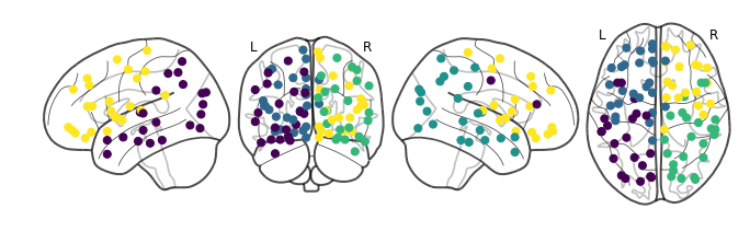
This command will output labels to our data points named spectral.labels_, we can use this to colorcode our data points! By using nilearn’s plot_connectome function, we can visualize our two groups in a brain:

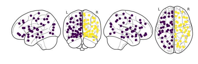
The spectral clustering function itself received no information regarding brain region locations, the algorithm was not given a set of labels and coordinates of each brain region. It was only given connection strengths between about 90 data points, but somehow it managed to separate the brain into left and right hemispheres!

Let’s see what clustering into four groups look like:

We are starting to see anterior and posterior separation! What about five:

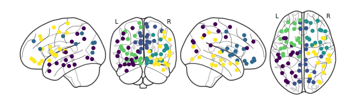
In addition to the four big lobes, we are starting to see functionally specialized regions being highlighted. The new group right in the middle of the two hemispheres include regions like the precuneus, occipital lobe, and the cingulum. These are some of the earliest identified brain structures with the heaviest wirings inside the brain.

Rubber band interpretation

So why does this grouping happen? The name spectral clustering comes from spectral graph theory, which is the study of a graph’s characteristic polynomials, or eigen values and eigen vectors of a graph. Remember when I mentioned graph Laplacians have “nice” eigen properties? All spectral clustering algorithms rely on these “nice” eigen properties.

In an ideal scenario where we want $k$ clusters of a similarity matrix $M$, where the data points in each $i$-th cluster $k_i$ have a similarity of 0 (no difference at all, exactly the same), then the eigen vectors of this $M$ will represent each cluster as:

\begin{bmatrix} 1 & 0 & … & 0\\ 0 & 1 & … & 0\\ \vdots & \vdots & \ddots & \vdots\\ 0 & 0 & … & 1 \end{bmatrix}

All clusters are distinctly different from each other, and all data points belonging to the same cluster $k_i$ will coincide to the $i$-th eigen vector. Any simple clustering algorithm can trivially separate these data points.

In the case of our brain connectivity ($C$), we are far from ideal, but we know this is some distance away from the ideal matrix $M$: $C = M + P$, where $P$ is a perturbation of the network that transforms $M$ to $C$. Now if we quantify the changes in eigen vectors and eigen values with the perturbation $P$, we can claim that the perturbed eigen vectors behave approximately the same as the ideal eigen vectors if the difference between the two is minimized. This is just the mathy way of saying, let’s stretch out this network of rubber bands, and observe if they can be stretched to our ideal scenario, and we will categorize these rubber bands based on our expected ideal scenario as best as we can.

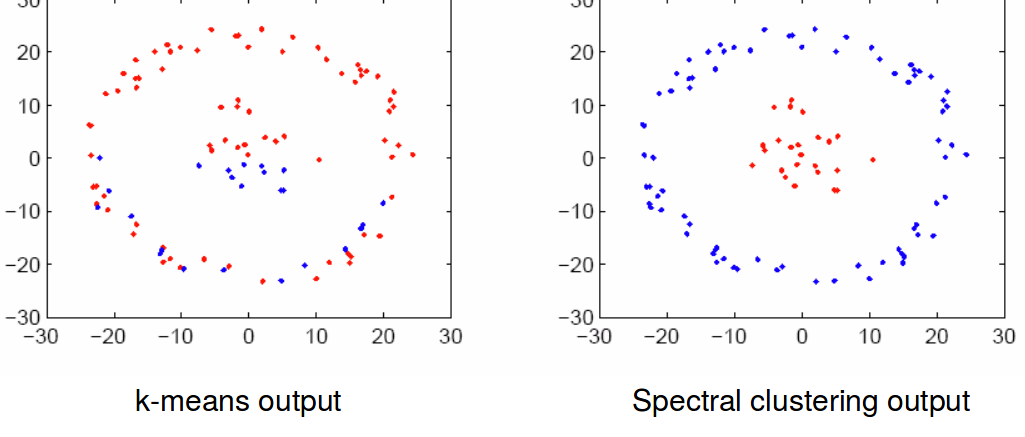
Spectral clustering and utilizing Laplacian eigen vectors is much more poweful than simply clustering data points as they are. Here’s a good example of k-means algorithm vs. spectral clustering, where the k-means algorithm fails to determine the best separation between the data points:

In spectral clustering, rather than computing the variances in a raw dataset, we use a dataset’s innate properties! We stretch the data around to see how it would react, and group them together based on their spectral properties. This methodology is extremely popular in machine learning, and has been extended to all sorts of data science settings. It’s a neat little tool to keep in every neuroscientist’s pockets.

Resources used while writing this post:

• The Lab post-doc Pablo Damasceno’s jupyter notebook on spectral clustering. He presented this metholody at a lab meeting first :).

• Von Luxburg, U. (2007). A tutorial on spectral clustering. Statistics and Computing, 17(4), 395–416. https://doi.org/10.1007/s11222-007-9033-z

• Ivković, M., Kuceyeski, A., & Raj, A. (2012). Statistics of weighted brain networks reveal hierarchical organization and gaussian degree distribution. PLoS ONE, 7(6), e35029. https://doi.org/10.1371/journal.pone.0035029