TensorFlow & probabilistic ML - Regression

The examples displayed here are taken from Kevin Murphy’s probabilistic machine learning Colab notebook. I found the code to be very instructive when paired with the math formulations, and thought I’d expand the logic here for people hoping to explore probabilistic modeling with tensorflow-probability.

Linear regression is a basic curve fitting technique using a straight line model to approximate the data trend. However, when the data is noisy, scientists need to understand the assumptions and quantify the reliability of their curve fitting methods. A probabilistic approach to modeling enables the quantification of uncertainty, but implementing this powerful approach is isn’t always straight forward for beginners, especially without knowledge of the available toolkits. We will first look at linear regression in it’s simplest form, and then create a Sequential model for the probabilistic approach.

The Data

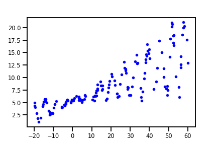
The 150 data points used here are synthesized with linear trend specified by w = 0.125 and b=5.0, or slope and intercept, respectively. We used numpy’s rand function to introduce some randomness in both the dependent and independent variables. The data is displayed below, a 1+sin(x) + noise scaling was used for the dependent variable y to create the dispersing noise effect.

Ordinary least squares linear regression

The most basic form of linear regression uses ordinary least squares, which aims to minimize the sum of squares between the observed data points and the predictions from the linear model.

This approach is implemented by scikit-learn’s LinearRegression module. And we can easily apply it to our data with the following:

from sklearn.linear_model import LinearRegression

reg = LinearRegression().fit(x, y) 
reg_line = x_tst * reg.coef_ + reg.intercept_ # linear model

# plot
plt.figure()
plt.plot(x, y, "b.", label="observed")
plt.plot(x_tst, reg_line, "r", label='OLS', linewidth=4)

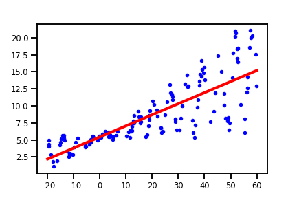
The fit() method will find the weights w and intercept b for the linear approximation $w\pmb{x} + b$ that minimizes the squared sum error. With LinearRegression, we can call the score() method to obtain a $R^2$ coefficient of determination. In this case, we obtained $\hat{w} = 0.16$ and $\hat{b} = 5.44$ with a $R^2$ coefficient of $0.66$. The model does a pretty decent job, but the $R^2$ coefficient doesn’t capture the uncertainty of 150 prediction by itself alone.

Probabilistic Regression Overview

The general approach is to obtain a conditional probability density $p$, based on some observed data $x$ and model parameters $\theta$. If we assume the probability density to be Gaussian shaped, then we will only have to worry about the mean and variance:

\begin{equation} p(y \mid \boldsymbol{x} ; \boldsymbol{\theta})=\mathcal{N}\left(y \mid f_{\mu}(\boldsymbol{x} ; \boldsymbol{\theta}), f_{\sigma}(\boldsymbol{x} ; \boldsymbol{\theta})^{2}\right) \end{equation}

where $f_{\mu}$ and $f_{\sigma}$ predict the mean and variance respectively.

With this formulation, we can already see one advantage of the probabilistic approach, we can make the variance depend on the input $\boldsymbol{x}$, which is called heteroskedastic regression. And assuming we are working with linear functions (linear regression), we have:

\begin{equation} p( y \mid \boldsymbol{x}; \boldsymbol{\theta}) = \mathcal{N}(y \mid \boldsymbol{w}_{\mu}^T \boldsymbol{x} + b, \operatorname{softplus}(\boldsymbol{w}_{\sigma}^{T} \boldsymbol{x} + b)) \end{equation}

with the “softplus” function: $\sigma_{+} (a) = \log (1 + e ^{a}) $, ensuring the predicted standard deviation is non-negative. And we are looking for the parameters $\boldsymbol{w_{\mu}},\boldsymbol{w_{\sigma}}, b$.

TensorFlow Code Explained

We can take advantage of tensorflow-probability’s probabilistic models and its flexibility to combine with layering capabilities from keras:

• Sequential: evaluates layers with one input and one output in sequence.
• Dense: our linear model output = activation(dot(input, weight)+bias), and we set activation=None, so this is equivalent to $wx + b$. The output becomes an input to the next layer in sequence.
• DistributionLambda: Takes the output from Dense as input to a callable function, and returns a TensorFlow probability Distribution instance. Usually one would have to sample the distribution to have a tensor output, but in our case, we want the output as a distribution to compute the log-likelihood cost function.

The full model code:

model = tf.keras.Sequential(
    [
        tf.keras.layers.Dense(2), # 2 outputs, 1 for mean, 1 for variance
        tfp.layers.DistributionLambda(
            lambda t: tfd.Normal(loc=t[...,:1], scale = tf.math.softplus(0.05 * t[..., 1:])) # first output for mean, second output for variance, this notation instead of [...,0], [...,1] preserves the output dimensions
        ),
    ]
)

You can use the model.summary() method for an overview of the structure and parameters in this model:

Model: "sequential_1"
_________________________________________________________________
 Layer (type)                Output Shape              Param #   
=================================================================
 dense_8 (Dense)             (None, 2)                 4         
                                                                 
 distribution_lambda_1 (Dist  ((None, 1),              0         
 ributionLambda)              (None, 1))                         
                                                                 
=================================================================
Total params: 4
Trainable params: 4
Non-trainable params: 0
_________________________________________________________________

The 4 parameters we are training for are the weights and biases for the two linear models. With the DistributionLambda layer, we are creating a Gaussian distribution output with a probability density function of the form:

\begin{equation} \mathcal{N}\left(y \mid \mu, \sigma^{2}\right) \triangleq \frac{1}{\sqrt{2 \pi \sigma^{2}}} e^{-\frac{1}{2 \sigma^{2}}(y-\mu)^{2}} \end{equation}

The model output distribution has a log_prob method, evaluating the log of the Gaussian’s probability density function at a given value, which is equivalent to the log-likelihood expression:

\begin{equation} \mathrm{NLL}\left(y | \boldsymbol{w}, \sigma^{2}\right)=-\sum_{n=1}^{N} \log \left[\left(\frac{1}{2 \pi \sigma^{2}}\right)^{\frac{1}{2}} \exp \left(-\frac{1}{2 \sigma^{2}}\left(y_{n}-\boldsymbol{\mu}\right)^{2}\right)\right] \end{equation}

So now we must figure out the values of $\mu$ and $\sigma^2$ that results in the maximum value of the above expression with respect to our observed data $y$. This is also known as the maximum likelihood estimation. I won’t go into the details here about the math of joint densities and differentiating the log-likelihood function, and instead focus on the simple code implementation in tensorflow:

# define negative log-likelihood cost function
# Recall that our model output is a Distribution with log_prob method.
# rv_y is the output Gaussian
# y is the observed data
negloglik = lambda y, rv_y: -rv_y.log_prob(y)

# Compile keras model with optimizer and cost function
model.compile(optimizer=tf.optimizers.Adam(learning_rate=0.01), loss = negloglik)

# fit() returns a history object with records of the cost function values during the model fitting process
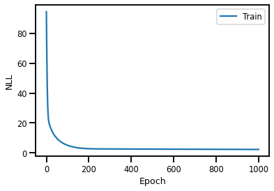
history = model.fit(x, y, epochs = 1000, verbose = False)

# visualize the parameter fitting:
plt.plot(history.history["loss"], label = "Train")
plt.legend()
plt.xlabel("Epoch")
plt.ylabel("NLL")
plt.show()

To see the newly optimized weights and biases:

model.weights

[<tf.Variable 'dense_1/kernel:0' shape=(1, 2) dtype=float32, numpy=array([[0.1395756 , 0.93267053]], dtype=float32)>,
 <tf.Variable 'dense_1/bias:0' shape=(2,) dtype=float32, numpy=array([ 5.665921, 12.169089], dtype=float32)>]

The results for the mean are in the first column, which are slightly different from the scikit-learn results from before. But we also have a separate set of weight and bias terms for the variance! We can visualize this heteroskedastic model:

yhat = model(x_tst) # evaluate the model with x_tst vector

plt.figure()
plt.plot(x, y, "b.", label="observed")
m = yhat.mean() # mean of the Gaussians
s = yhat.stddev() # variance of Gaussians

plt.plot(x_tst, m, "r", linewidth=4, label="mean")

# plot uncertainty with approximated 95% confidence interval
plt.plot(x_tst, m + 2 * s, "g", linewidth=2, label=r"mean + 2 stddev")
plt.plot(x_tst, m - 2 * s, "g", linewidth=2, label=r"mean - 2 stddev")

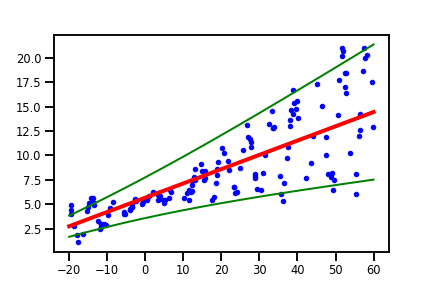
The plot above includes lines of $\mu \pm 2\sigma(x)$, which are $95\%$ interval approximations, illustrating uncertainty in our model predictions given $x$, which takes into account the variability in our data. Of course, there is a variation with homoskedastic variance, and the uncertainty captured in the Gaussian distributions will be from the estimated parameters. But the main take-away is that the probabilistic approach enables the quantification of variance and uncertainty!

Once again, the full example can be seen in the Colab notebook, which has the homoskedastic implementation as well. Feel free to play around and see how the $\sigma^2$ term changes based on different scaling. The math behind maximum likelihood estimation is covered in numerous online resources, but @SirBayes’s textbooks are an excellent resource for probability foundamentals and machine learning math. I hope to review & share more topics from these books and use the code examples as an additional learning tool.